
Under construction
Images are available in full resolution for download here as well as in this gallery and this zip file with all of these in one file. The zip file also contains additional measurements for the case I've shortcutted one of the wire ends to ground and terminated the other with 500 ohms, which resulted in considerable reflections. There's a readme.txt file describing what I've done. Discussion and/or comments can be made on ResearchGate.
Abstract
In 1834, Charles Wheatstone measured the velocity of electricity along two long wires, whereby he found a velocity of about 463,500 km/s, over 1.5 times the speed of light. In 1905, Nikola Tesla also measured a propagation speed for the telluric currents he transmitted trough the earth's surface of 471,240 km/s, remarkably close to Wheatsone's result and within 0.1% of pi/2 times the speed of light.
In order to validate the possibility of transmitting superluminal signals along a wire, we setup an experiment, similar in design to Wheatstone's, consisting of two relatively long wires which were excited by a capacitive discharge. Hereby, a mercury wetted relay was used as a switching element in order to obtain as fast a signal rise time as possible.
Quite surprisingly, the superluminal signal was detected and found to propagate at more than 1.8 times the speed of light. This is quite a lot faster than the theoretical pi/2 (1.57), which may be caused by the use of enamelled wire rather than unshielded wire.
Introduction
Characteristic for this setup was that the wires operated as a single wire transmission line, which can be described as a distributed series LC circuit. This is the kind of transmission line Tesla was working with, which has been all but forgotten because the superluminal longitudinal waves propagating along such a transmission line are not supported by Maxwell�s equations. The behavior of the single-wire transmission line is significantly different from the familiar dual wire transmission line, which can be described as a distributed parallel LC circuit.
Methods
The schematic for the setup is rather simple. A 100 nF capacitor is switched between a 5V power supply and two rather long wires by a mercury wetted relay with double contacts:
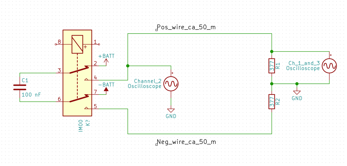
The relay was switched on/off about once every second by means of a standard 555 timer circuit (not shown). The rise time of this circuit while connected to the long wires was measured using an oscilloscope with an active probe (channel 1) as well as a capacitively coupled 1:10 passive probe (channel 2):
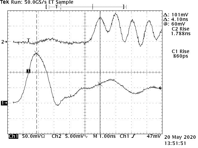
The measured rise time was 860 ps, but it may be even faster since the measured rise time may actually be the limit of what the active probe can handle. The same signal measured with a passive probe resulted in an delay of 4.1 ns because of a longer coaxial cable connecting the probe to the scope. The oscilloscope has a maximum sampling rate of 100 Ms/s, so in order to obtain an effective sampling rate of 50 Gs/s, as shown in this measurement, the signal has to be repeated multiple times. For a resolution as high as in this measurement, several hundreds of measurements were peformed, which took about half an hour. Given the smoothness of the signals measured this way, it is clear that the repeatability of the signals is excellent and the use of a mercury wetted relay is very effective for eliminating contact bounce.
The circuit around the relay is shown in the following photograph at the left, whereby a passive probe is shown to be capactively coupled to the wire connected to the positive lead of the capacitor. And the termination resistor circuit is shown at the right, along with an active probe and a passive probe, the latter of which is shown to be capacitively coupled to the wire connected to the positive lead of the capacitor:
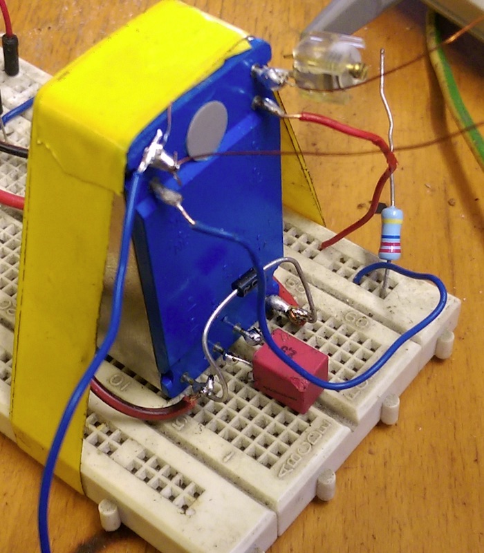
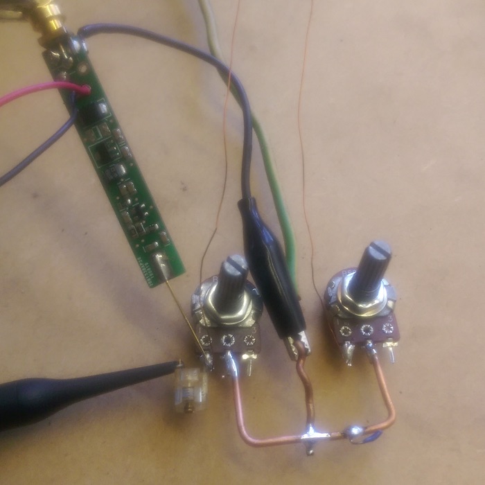
The ends of the wires are both terminated with a resistor (potentiometer) of about 375-380 ohms to earth ground, which is also the point where the ground lead from the scope was connected via the ground lead of one of the probes. Earth ground consisted of a metal rod of a few meters in length, which was placed vertically into the ground just outside the shack and connected to a 1.5 mm^2 standard electrical insulated wire, perhaps 2-3 m in length, with yellow/green markings as is visible on the photograph.
The resistance of about 377 ohm was chosen to match the characteristic impedance of free space, which is also the impedance Elmore found for the guided EM surface wave he was able to transmit along an unshielded wire, very similar to the better known Goubau line.
An overview of the measurement setup is shown in the following photograph:
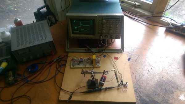
Channel 1 of the scope is connected to the active probe. Channel 2 is a passive 1:10 probe used for triggering and is connected to the positive lead of the capacitor, via a 10 pF trimmer as coupling capacitor. Channel 3 is also a passive 1:10 probe, with which the signal from the active probe can be compared. At the end of the positive wire, there's also a 10 pF coupling trimmer, so one can opt for capacitive coupling at that point as well. It should be noted that other experiments aimed at attempting to emit longitudinal waves from a dipole suggested it works best to use foil trimmers or tuning capacitors with air as a dielectric, while fixed ceramic capacitors did not seem to work as expected.
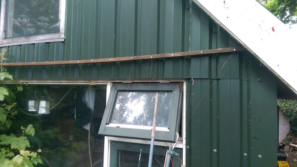
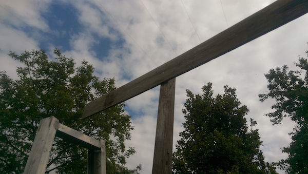
Two enamelled copper wires of 0.25 mm diameter were hung up at a height of about 2 m above ground. The distance between the shack and the supporting pole is 12.5 m and both wires go back and forth two times, giving a length of just over 50 m each. The distance between two adjacent pieces of the wires was about 10-20 cm. In addition, the wires were led into the shack. The one connected to the positive terminal of the capacitor is about 54.8 m long and the one to the negative terminal 54.1 m, both +/- 20 cm or so.
It seems that the influence of the probes to the circuit is minimal, but the bandwidth of the active probe certainly makes a difference in obtaining clear signals.
Measurements
The following pictures contain the scope shots of what was measured. They are in chronological order and under each picture, there's a short note on the timing feature that was measured as well as a time stamp on when the measurement took place:
Channel 1 on the negative wire, gnd via passive probe, FTL edge 96 ns, 14:12
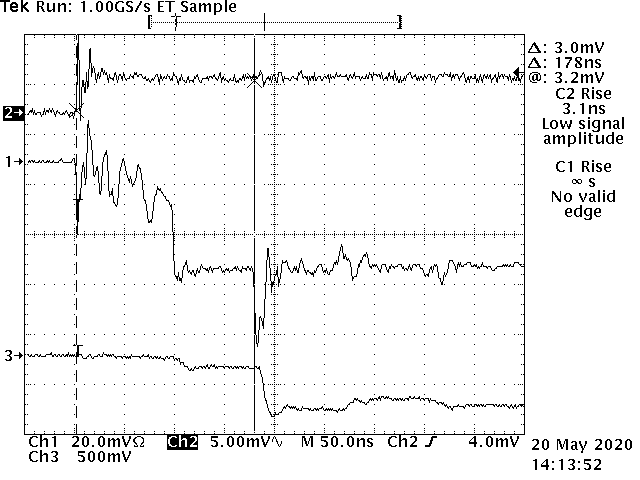
Channel 1 on the negative wire, gnd via passive probe, EM edge 178 ns, 14:13
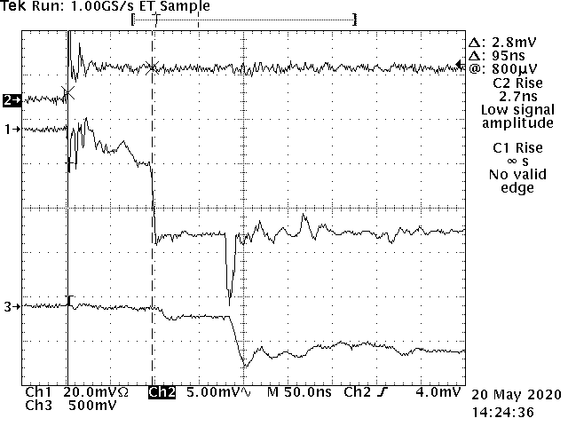
Channel 1 on the negative wire, gnd via active probe, FTL edge 95 ns, 14:24
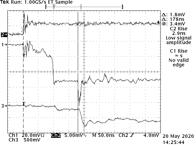
Channel 1 on the negative wire, gnd via active probe, EM edge 178 ns, 14:25
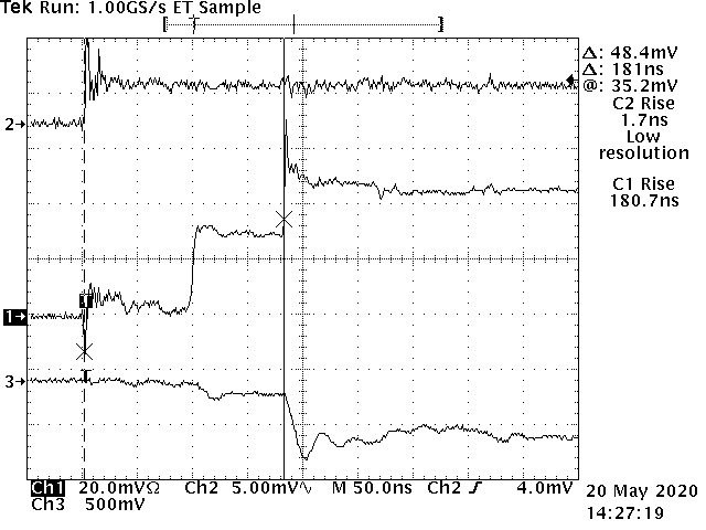
Channel 1 on the positive wire, EM edge 181 ns, 14:27
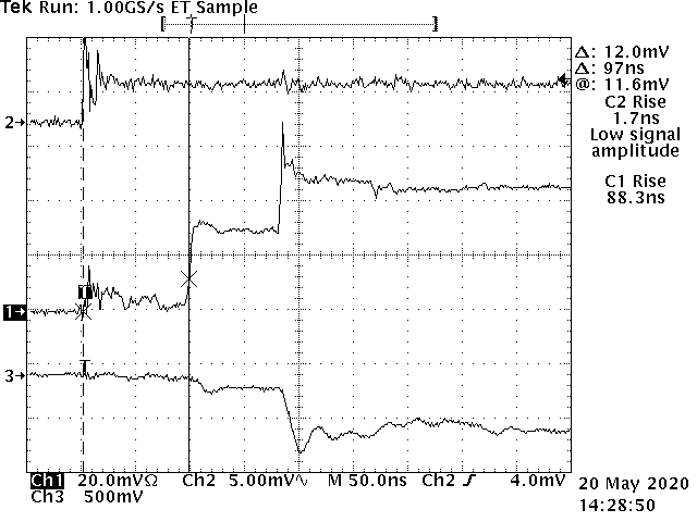
Channel 1 on the positive wire, FTL edge 97 ns, 14:28
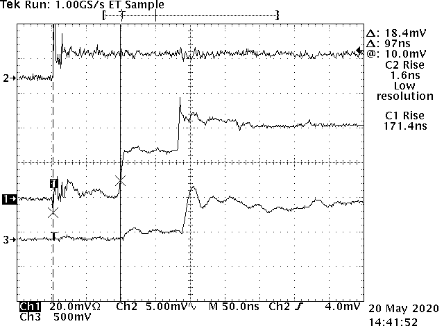
Channel 1 on the positive wire, FTL edge 97 ns, 14:41
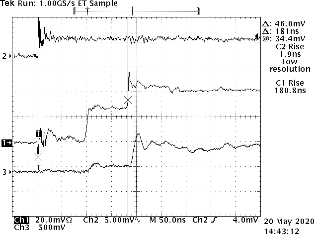
Channel 1 on the positive wire, EM edge 181 ns, 14:43
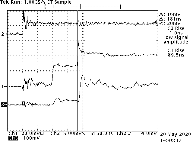
Channel 1 on the positive wire, Channel 3 capacitively coupled, EM edge 181 ns, 14:46
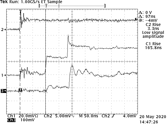
Channel 1 on the positive wire, Channel 3 capacitively coupled, FTL edge 97 ns, 14:47
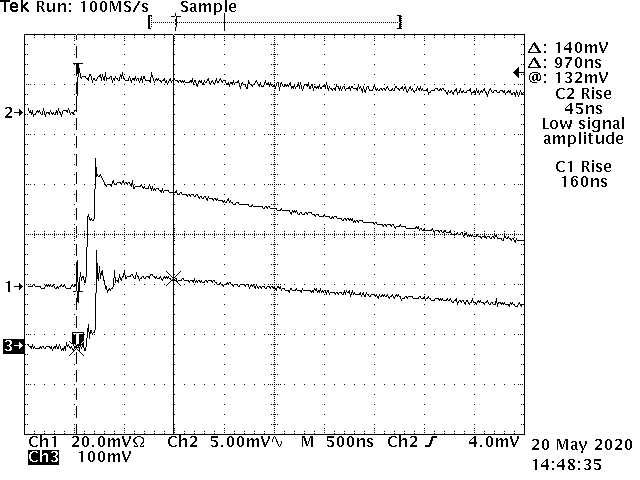
Channel 1 on the positive wire, Channel 3 capacitively coupled, 100 Ms/s overview, 14:48
Equipment
- Oscilloscope: Tektronix TDS460A digitizing oscilloscope. Serial # B070978. Last calibrated 2006-49.
- Active probe: 60dbm.com. This probe has an attenuation of approximately 20 dB over a bandwidth of 100 kHz - 1.5 Ghz. The probe is capacitively coupled and has an imput impedance of about 0.75 pF in series with a 10 MOhm resistor.
- Mercury wetted relay: CP Clare HGS2M 50051.
- Multimeter: Voltcraft VC 820.
Notes and further research
This is part of an email I sent to Simon Derricut with some further ideas and detals I still need to write out properly in the above text:
Yes, the ADC('s?) can only do 100 Ms/s, so the signal has to be repeated quite a lot of times in order to obtain a full picture. It seems the timing circuitry of the scope is excellent, it can do up to 50 Gs/s in "extended time", which I've used to measure the risetime of the signal. Since I'm steering the relay about once a second, this took quite a while, half an hour or so.
I've been working on an article to write things up. It's far from finished, but I included a schematic:
I'm thinking about doing some additional experiments. First of all, I want to repeat the experiment with unshielded wires, because I suspect the FTL wave will be slower then. Would be nice if it were, because then we gained some significant insight and can also pretty much rule out coupling between the wires causing some artifact. I have about 100 m of titanium wire of 0.08 mm diameter, which would minimize capacitive coupling, as Milnes argued:
According to this, the characteristic impedance of a transmission line is 276 * log(d/r):
https://www.allaboutcircuits.com/textbook/alternating-current/chpt-14/characteristic-impedance/
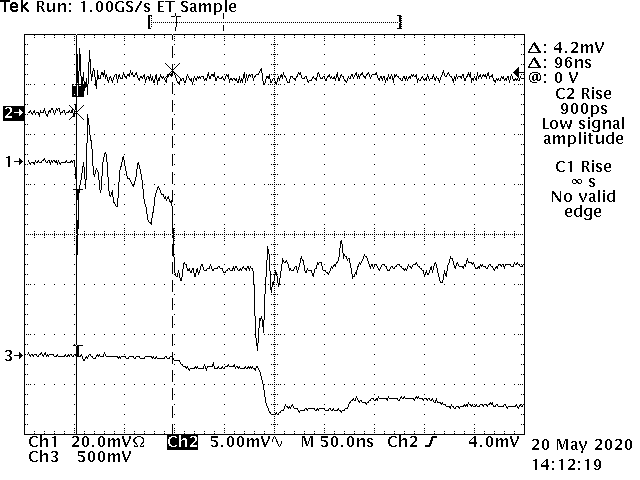
If the lines are about 10 cm apart, this works out to 1654 Ohms for the .25 mm diameter wire and 1968 Ohms for the .08 mm diamater wire. I've already played with the terminating resistors and adjusted them such that the reflections became minimal and a nice slope was obtained, such as in this picture:
When I measured the resistance, it came out at about 385 Ohms, which is very close to the 377 Ohms of free space and suggests we have Elmore's mode for the EM wave propagating along the wire and the wires are not acting as a dual wire transmission line. In this mode, the energy is contained within a few mm around the wire, according to Elmore:
"The field solutions show that the magnitude of the radial component follows a 1/r curve and that the majority of the propagated energy is within a few conductor diameters of the center axis."
Secondly, I want to experiment a bit further with this circuit:
https://www.epanorama.net/circuits/tdr.html
Would like to create a balanced version, whereby I have two outputs out of sync. This way, you don't inject a signal into the common ground, which reduces artifacts transmitted trough the ground leads.
Thirdly, I want to experiment further with trying to obtain a reflection of the FTL signal on the end of the wires. �Problem is I need to ground things somewhere, because otherwise the scope is not of much use. I'm thinking about putting two 100 nF capacitors in series rather than just one and then ground the connection in the middle. If I can get that to work, I can put the wires in a straight line in open space and eliminate any possibility of capacitive coupling between two adjacent wires.�
All in all, there's still quite a lot of work to do, but so far I've found the results very encouraging.