
An exceptionally elegant "Theory of Everything"
By Arend Lammertink, MScEE, October 2016.
lamare {at} gmail [dot] com
Update: This work has been rewritten and extended into a draft scientific paper, which may or may not be published in a scientific journal some day.
Abstract
In a previous article, we stated that all currently known areas of Physics' theories converge naturally into one Unified Theory of Everything once we make one fundamental change to Maxwell's aether model. In that article, we explored the history of Maxwell's equations and considered a number of reasons for the need to revise Maxwell's equations. So, if you're more interested in an intuitive explanation, you may want to start there.
In this article, we will make the mathematical case that there is a hole in Maxwell's equations which should not be there, given that we started with the same basic hypothesis as Maxwell did:
A physical, fluid-like medium called "aether" exists.
Maxwell did not explicitly use this underlying hypothesis, but abstracted it away. This leads to a mathematically inconsistent model wherein, for example, units of measurements do not match in his definition for the electric potential field. That is: when considering these units of measurements as they would have when derived from a basic aether model. By correcting this obvious flaw in the model and extending it with a definition for the gravity field, we obtain a simple, elegant, complete and mathematically consistent "theory of everything" without "gauge freedom". And since gauge theory forms the theoretical basis for Quantum Field Theory, we must reject both as a basis for Theoretical Physics.
Paul Stowe's Aether model
In their paper The Atomic Vortex Hypothesis, a Forgotten Path to Unification (2013), Paul Stowe (see sidebar) and Barry Mingst provided a remarkable basis for come to a "Theory of Everything", an accomplishment which was not Einstein's lot to find. Their conclusions:
In our previous article, however, we discovered that Maxwell did not actually use this "atomic vortex hypothesis" in his model, other than using it as an analogy. Maxwell abstracted the actual vorticity of the magnetic field and the medium away by defining only the resulting magnetic field {$\mathbf{B}$} and keeping the magnetic vector potential {$\mathbf{A}$} undefined. As we shall see, it is this "hole" in Maxwell's equations which led to numerous attempts to tape the hole over, from relativity all the way to currently popular Quantum Weirdness. In other words:
For the past hundred+ years, science has repeatedly attempted to extend the model with the popular duck-tape/chewing-gum of the decade, rather than correcting the model for an, in hindsight, obvious flaw: Maxwell's hole.
In the following, we shall consider how and where this hole can be found. Let us begin by following Stowe and define a vector field analogue to fluid dynamics, using the continuum hypothesis:
We define this vector field P as:
{$$ \mathbf{P}(\mathbf{x},t) = \rho(\mathbf{x},t) \mathbf{v}(\mathbf{x},t), $$}
where x is a point in space, $\rho(\mathbf{x},t)$ is the averaged aether density at x in [kg/m3] and $\mathbf{v}(\mathbf{x},t)$ is the local bulk aether flow velocity at x in [m/s].
With this, we can apply textbook fluid dynamics vector theory in order to derive field and potential equations from the local bulk aether flow velocity vector field $\mathbf{v}(\mathbf{x},t)$, or {$\mathbf{v}$} for short.
Helmholtz decomposition
Let us now consider the Helmholtz decomposition:
The physical interpretation of this decomposition, is that the a given vector field can be decomposed into a longitudinal and a transverse field component:
It can be shown that performing a decomposition this way, indeed results in the Helmholtz decomposition. Also, a vector field can be uniquely specified by a prescribed divergence and curl:
{$$ \nabla \cdot \mathbf{F_v} = d \text{ and } \nabla \times \mathbf{F_v} = \mathbf{C} $$}
This is confirmed in Bioelectromagnetism - Principles and Applications of Bioelectric and Biomagnetic Fields by Jaakko Malmivuo & Robert Plonsey:
And in The Helmholtz Theorem and Superluminal Signals by V.P. Oleinik it is stated:
The "Laplacian"
Let us now consider the Laplacian:
[...]
{$$ \Delta f = \nabla^2 f = \nabla \cdot \nabla f $$}
It should be no surprise that the Laplacian of a scalar field {$\psi$} is defined exactly the same, as the divergence of the gradient:
{$$ \nabla^2 \psi = \nabla \cdot (\nabla \psi) $$}
And since the divergence gives a scalar result, the Laplacian of a scalar field also gives a scalar result.
When we equate the Laplacian to 0, we get Laplace's equation:
{$$ \nabla^2 \phi=0 $$}
It is also used in the Wave equation {$$ \nabla^2 \psi=\frac{1}{v^2}\frac{\partial^2\psi}{\partial t^2} $$}
Vector Laplacian
The (scalar field) Laplacian concept can be generalized into vector form, the Vector Laplacian:
{$$ \nabla^2 \mathbf{F} = \nabla(\nabla \cdot \mathbf{F}) - \nabla \times (\nabla \times \mathbf{F}) $$}
Deriving "Maxwell's" equations from the first order Laplacian
Application of the vector Laplacian to the local bulk aether velocity vector field {$\mathbf{v}$} gives:
{$$ \nabla^2 \mathbf{v} = \nabla(\nabla \cdot \mathbf{v}) - \nabla \times (\nabla \times \mathbf{v}) $$}
Now let us work this out by writing out the above terms in their components and giving these their familiar names and historic signs. Thus, we define a vector field {$\mathbf{A}$} for the magnetic potential, a scalar field {$\Phi$} for the electric potential, a vector field {$\mathbf{B}$} for the magnetic field and a vector field {$\mathbf{E}$} for the electric field by:
{$$ \mathbf{A} = \nabla \times \mathbf{v} $$} {$$ \Phi = \nabla \cdot \mathbf{v} $$}
{$$ \mathbf{B} = \nabla \times \mathbf{A} = \nabla \times (\nabla \times \mathbf{v}) $$} {$$ \mathbf{E} = - \nabla \Phi = - \nabla (\nabla \cdot \mathbf{v}) $$}
According to the Helmholtz theorem, {$ \mathbf{v} $} is uniquely specified by {$\Phi$} and {$\mathbf{A}$}. And, since the curl of the gradient of any twice-differentiable scalar field {$ \Phi $} is always the zero vector, {$\nabla \times ( \nabla \Phi ) = \mathbf{0}$}, and the divergence of the curl of any vector field {$\mathbf{A}$} is always zero as well, {$\nabla \cdot ( \nabla \times \mathbf{A} ) = 0 $}, we can establish that {$\mathbf{E}$} is curl-free and {$\mathbf{B}$} is divergence-free, and we can write:
{$$ \nabla \times \mathbf{E} = \mathbf{0} $$} {$$ \nabla \cdot \mathbf{B} = 0 $$}
For the summation of {$ \mathbf{E} $} and {$ \mathbf{B} $}, we get:
{$$ \mathbf{E} + \mathbf{B} = - \nabla (\nabla \cdot \mathbf{v}) + \nabla \times (\nabla \times \mathbf{v}) = - \nabla^2 \mathbf{v}, $$}
which thus gives the negated vector Laplacian for {$ \mathbf{v} $}.
Since {$\mathbf{v}$} is uniquely specified by {$\Phi$} and {$\mathbf{A}$}, and vice versa, we can establish that with this definition, we have eliminated "gauge freedom". This clearly differentiates our definition from the usual definition of the magnetic vector potential, which is defined along with the electric potential ϕ (a scalar field) by the equations:
{$$ \mathbf {B} =\nabla \times \mathbf {A} \,,\quad \mathbf {E} =-\nabla \phi -{\frac {\partial \mathbf {A} }{\partial t}} $$}
[...]
With our definition, we cannot add curl-free components to {$ \mathbf{v} $}, not only because {$ \mathbf{v} $} is well defined, but also because such additions would essentially be added to {$ \Phi $}, which encompasses the curl-free component of our decomposition.
With our definition, we can also establish units of measurement for the defined fields, since the local bulk aether flow velocity vector has a unit of measurement of meters per second [m/s]. For the electric potential {$\Phi$} we get per second [/s], for the magnetic potential {$\mathbf{A}$} we get radians per sec [rad/s], and for the electric and magnetic fields we get per meter second [/ms].
Now let us consider the difference between our definition and the textbook definition for electric potential:
{$$ \mathbf {E} =-\nabla \phi -{\frac {\partial \mathbf {A} }{\partial t}} $$}
For the term {$\frac {\partial \mathbf {A} }{\partial t}$}, we get a unit of measurement of radians per second squared [rad/s^2], while the electric field has a unit of measurement in [/ms]. These obviously do not match, which means Maxwell's definition for the electric potential is mathematically inconsistent.
So, Maxwell's implicit use of the aether model not only introduced an unwarranted "gauge" freedom to the model, he also introduced an unwarranted and inconsistent time derivative of the magnetic potential to his electric field definition. And this is exactly why Maxwell's equations were found not to be invariant to the Galilean coordinate transform and thus a new coordinate transform had to be found in order to "correct" for this time derivative which should not even have been there in the first place. Well, that new transform was the Lorentz transform and the rest is history.
Deriving gravity from the second order Laplacian
In an e-mail Paul Stowe sent me, he wrote:
As Koen van Vlaenderen pointed out, it does not make sense to take the gradient of a gradient, but the idea that gravity should be naturally included in our aether model in the form of a field derived from the electric field makes a lot of sense. This is also supported by experimental data around the Biefeld�Brown effect, even though recent confirmation attempts by Martin Tajmar yielded a null result.
Further, considering the wave-particle duality principle which states that particles are electromagnetic in nature, there can be no other fundamental forces of nature but the electromagnetic and therefore gravity must be derived from the field definitions for the electromagnetic fields.
In other words: the most logical approach to define gravity is to derive it from the electric field, completely analogous to the way we derived the electromagnetic fields from our bulk aether flow velocity field, namely by working our the second order Laplacian for v, which would be the Laplacian for E.
And since the electric field is defined to be curl free, the Laplacian for the gravity field is given by:
{$$ \nabla^2 \mathbf{E} = \nabla (\nabla \cdot \mathbf{E}) = - \nabla (\nabla \cdot (\nabla (\nabla \cdot \mathbf{v})) ) $$}
Now let us work this out by writing out the above by defining a scalar field {$V$} for the gravitational potential and a vector field {$\mathbf{G}$} for the gravitational field by:
{$$ V = \nabla \cdot \mathbf{E} $$} {$$ \mathbf{G} = \nabla V = \nabla (\nabla \cdot \mathbf{E}) $$}
And since {$\mathbf{G}$} is curl-free we can write:
{$$ \nabla \times \mathbf{G} = \mathbf{0} $$}
This way, gravity is described as being standing longitudinal waves. And as you would expect, this matches exactly to experimental data in so called Cymatics experiments, which show how this works in water and other fluids. This picture makes clear that gravity should indeed be considered to be standing longitudinal waves:
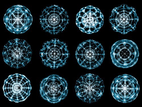
By now it should be clear that the combination of gravity, longitudinal standing waves, and magnetism, curl or vorticity, are the dominant phenomena responsible for shaping atoms, molecules, solar systems, galaxies, etc., etc.
Theory of everything??
With this simple approach, we have already established that gravity is not a fundamental interaction or force. However, two other fundamental interactions have been defined, the "weak" and "strong" nuclear forces.
However, from Stowe's theory as well as the wave-particle duality principle, we know that particles are electromagnetic in nature. And since this is the case, no other fundamental forces but the electromagnetic can exist. And, it can be shown in the laboratory that magnetic forces are actually responsible for maintaining the geometry and shape of atom nuclei as well as their electron clouds, as has been done by David LaPoint:
Watch on YouTube, starting at 19:43
Herewith, we have established that with the equations derived above, we have indeed come to a complete "field theory of everything" covering all known fundamental forces of nature, namely the electromagnetic.
Now let us consider what a Theory of everything is considered to be:
Our theory undoubtedly qualifies as being "a theoretical framework revealing a deeper underlying reality" and it is also "a single theory that, in principle, is capable of describing all phenomena" and therefore it qualifies for being called a "Theory of everything", especially since it is also testable. Paul Stowe and Barry Mingst have already shown that with this framework, a number of anomalies can be resolved and we propose a number of experiments as well.
Furthermore, in our background article, we have explored the history of how the current standard model came to be and explained the fundamental ideas which led to the discovery of "Maxwell's hole" and explained how the "mutually incompatibility" between GR and QFT traces right back to "Maxwell's hole" as well as how this led to the concept of "compressibility of the medium" having been expressed by GR in the form of "compressibility of time".
In other words: we have proposed that with a simple and straightforward revision to the foundational framework of the standard model, Maxwell's equations, we can naturally reveal a deeper underlying reality which, in principle, is capable of describing all phenomena.
Isn't this in contradiction to Maxwell's theory?
Since our model is a revision of Maxwell's, it's obviously not the same. So, in that sense, one can say it's a non-Maxwellian model. In practice, however, the field definitions should lead to the same predictions as Maxwell's insofar as currently "empirically verified'. And no, we have not yet worked out c.q. shown how our definitions relate to Maxwell's. Our model promises to solve a fundamental problem we have identified in Maxwell's model, which we refer to as the "recursive problem".
In our historical background article this problem is referred to as a "non sequitur" issue:
So, what we argue is that our approach does not contradict Maxwell's theory (insofar as empirically verified), because the concept of "charge", being a property of certain particles, should be introduced at the particle modelling level and NOT at the medium modelling level.
In other words: because we have identified a recursive problem in the logical inter-relations between Maxwell's charge definition and that of "particles" or "photons", the concept of charge should not be included in the field model for logical reasons.
It should also be noted that, despite the Maxwell equations only describing one type of electromagnetic waves, actually at least two types of electromagnetic wave phenomena are known to exist, namely the "near" and the "far" field. Since our theory predicts transverse surface waves as well as expanding vortex rings to exist, it is clear that, at least in this regard, our theory promises to explain this phenomenon in a natural way, while Maxwell's theory does not predict it at all.
More on this in the FAQ.
Conclusions
By working out standard textbook fluid dynamic vector theory for an ideal, compressible, non-viscous Newtonian fluid, we have established that Maxwell's equations are mathematically inconsistent, given that these are supposed to describe the electromagnetic field from the aether hypothesis. Since our effort is a direct extension of Paul Stowe and Barry Mingst' aether model, we have come to a complete mathematically consistent "field theory of everything". And we found "Maxwell's hole" to be the original flaw in the standard model that led to both (Special and General) Relativity as well as Quantum Mechanics, which should thus both be rejected.
Notes and FAQ
Abstract posted at LinkedIn, thunderbolts.info and energeticforum.com.