
TESLA, PHYSICS AND ELECTRICITY
Research into the works of Nikola Tesla reveals electric phenomena that behave contrary to the theory of electricity in present use. Explanation of Tesla's inventions has been given from the standpoint of physics, yielding many misconceptions. The science of physics is based on the phenomena surrounding particles and mass, which finds little application in the study of electric phenomena.
The explanation of Tesla's discoveries are to be found in the science of electricity rather than the science of physics. The sci�ence of electricity has been dormant since the days (1900) of Stein�metz, Tesla and Heaviside. This is primarily due to vested interests which we may call the "Edison Effect." This material serves as a preface to a theoretical investigation of N. Tesla's discoveries by the examination of the rotating magnetic field and high frequency transformer. It is assumed that the reader is acquainted with the commonly available material on Tesla, and possesses a basic knowledge of mechanics and electricity.
THE ROTATING MAGNETIC FIELD
In the general electromechanical transformer energy is exchanged between mechanical and electric form. Such an apparatus typically employs a system of moving inductance coils and field magnets. It is desirable that the mechanical energy produced or consumed by of ro�tational form in order to operate with pumps, engines, turbines, etc. The method of producing rotary force, without the use of mechanical rectifiers known as commutators, was discovered by Nikola Tesla in the late 1800s and is known as the rotating magnetic field.
ELEMENTAL PRINCIPLES
An examination of the rudimentary interaction between inductance coils and field magnets will provide some insight into the principles behind the rotary magnetic field.
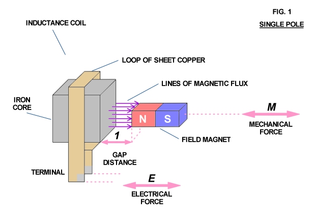
Consider a simple electromechanical device consisting of a piece of iron with a copper loop winding around it along with a small bar magnet (Fig. 1). Any variation in the distance (l) between the pole faces of the inductance coil and magnet produces an electromotive force (voltage) at the terminals of the copper loon resulting from the field magnet's lines of force passing through the iron core of the inductance coil. The magnitude of this E.M.F. is directly propor�tional to the speed at which the distance (l) is varied and the quan�tity of magnetism issuing from the field magnet pole face.
Conversely, if an electromotive force is applied to the induc�tance coil terminals, the distance (l) varies at a speed directly proportional to the strength of the E.M.F. and the quantity of magnet�ism issuing from the field magnet pole face. Thus electrical force and mechanical force are combined in this device.
If a flow of electrical energy (watts) is taken from the coil terminals and delivered to a load mechanical resistancy (friction) appears at the field magnet as a result of magnetic attraction and repulsion between the magnet and iron core. Mechanical force applied to the field magnet in order to move it results in power flow out of the coil. This flow of power generates an oppositional or counter electromotive force which repels the field magnet against the mechan�ical force. This results in work having to be expended in order to move the magnet. However this work is not lost but is delivered to the electric load.
Conversely, if the field magnet is to deliver mechanical energy to a load, with an externally E.M.F. applied to the coil terminals, the field magnet tends to be held stationary by the resistancy of the connected mechanical load. Since the field magnet is not in motion it cannot develop a counter E.M.F. in the coil to meet the externally applied E.M.F. Thus electrical energy flows into the coil and is de�livered to the field magnet as work via magnetic actions, causing it to move and perform work on the load.
Hence, mechanical energy and electrical energy are rendered on and the same by this electromechanical apparatus. Connecting this apparatus to a source of reciprocating mechanical energy produces an alternating electromotive force at the coil terminals, thus a linear or longitudinal A.C. generator. Connecting this apparatus to a source of alternating electric energy produces a reciprocating mechanical force at the field magnet, thus a linear A.C. motor. In either mode of operation the field magnet reciprocates in a manner not unlike the piston of the internal combustion engine. Rotary motion is not possible without the use of a crankshaft and flywheel.
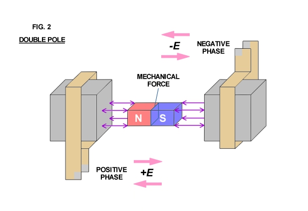
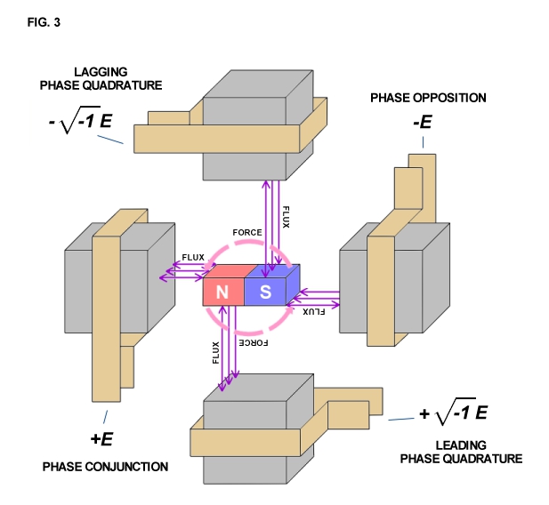
Arranging two inductance coils in a line as shown in Fig. 2 and connecting these coils to a pair of alternating E.M.F.s that are out of step by 1/2 of an alternating cycle with respect to each other results in the mechanical force being directed inwardly into the molecular spaces (inner space) within the field magnet. The field magnet is alternately stretched and compressed by magnetic action and no external force is evident except as vibration and heat. However, arranging two of the pairs shown in Fig. 2 at right angles to each other, connecting each to a pair of alternating E.M.F.s that are out of phase or step by one quarter cycle (quadrature) with respect to each other produces a rotating travelling wave of magnetism, that is, a whirling virtual magnetic pole.
This virtual pole travels from one pole face to the next during the time interval of one quarter cycle, thus making one complete revolution around all the pole faces for each cycle of alternation of the E.M.F.s. The field magnet aligns with the virtual pole, locking in with the rotary magnetic wave, thereby producing rotational force.
An analogy may assist in understanding this phenomena. Consider that the sun appears to revolve around the earth. Imagine the sun as a large magnetic pole and your mind's view of it as the field magnet. As the sun sets off in the distant horizon, it seemingly disappears. However, the sun is not gone but it is high noon 90 degrees, or one quarter, the way around the planet. Now imagine moving with the sun around the planet, always keeping up with it so as to maintain the constant appearance of high noon. Thusly, one would be carried round and round the planet, just as the field magnet is carried round and round by the virtual pole. In this condition the sun would appear stationary in the sky, with the earth flying backwards underfoot. Inspired to thinking of this relation by the poet Goethe, Tesla per�cieved the entire theory and application of alternating electric ener�gy, principally the rotating magnetic wave.
"The glow retreats, done is the day of toil; it yonder hastes, new fields of life exploring; Ah, that no wing can lift me from the soil, upon its track to follow, follow soaring..."
ROTATIONAL WAVES
The fundamental principle behind the production of the rotary magnetic field serves as the principle behind all periodic electric waves. It is therefore of interest to investigate the discovery a little further.
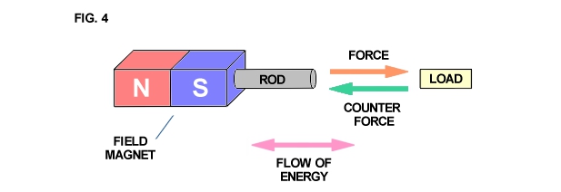
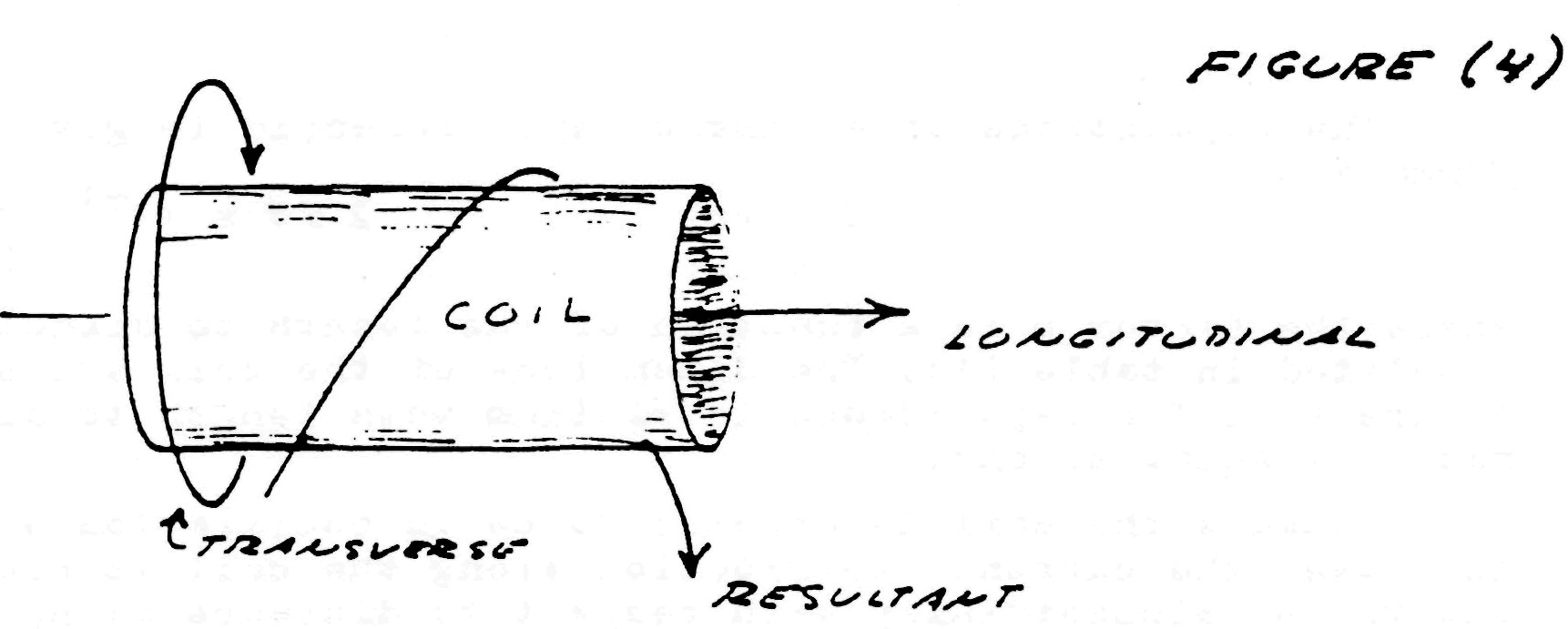
The apparatus shown in Fig. 1 develops mechanical force along the axis of the field magnet as shown in Fig. 4. Likewise, mechanical counterforce is applied along the axis of the field magnet. Hence, if work is to be drawn or supplied respectively to the field magnet from an external apparatus, a connecting rod is required between the two machines. The flow of energy is along the axis of the rod and thus is in line (space conjunction) with the forces involved. A simple analogy is a hammer and nail. The hammer supplies mechanical force to the nail, the nail transmitting the force into the wood. The counter-force tends to make the hammer bounce off the nail. However, the wood is soft and cannot reflect a strong counterforce back up the nail and into the hammer. Thus the nail slides into the wood absorbing mech�anical energy from the hammer which is dissipated into the wood.
The apparatus of Fig. 2 develops mechanical force axially also, but it is entirely concentrated within the molecular space. Any counterforce must push back along the same axis. Thus the work is also along axis like Fig. 4 and is delivered to the molecular struc�ture. The analogy is two hammers striking a steel block from op�posite sides, pounding the block and producing heat and vibration within it.
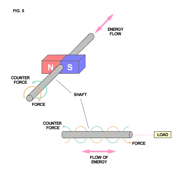
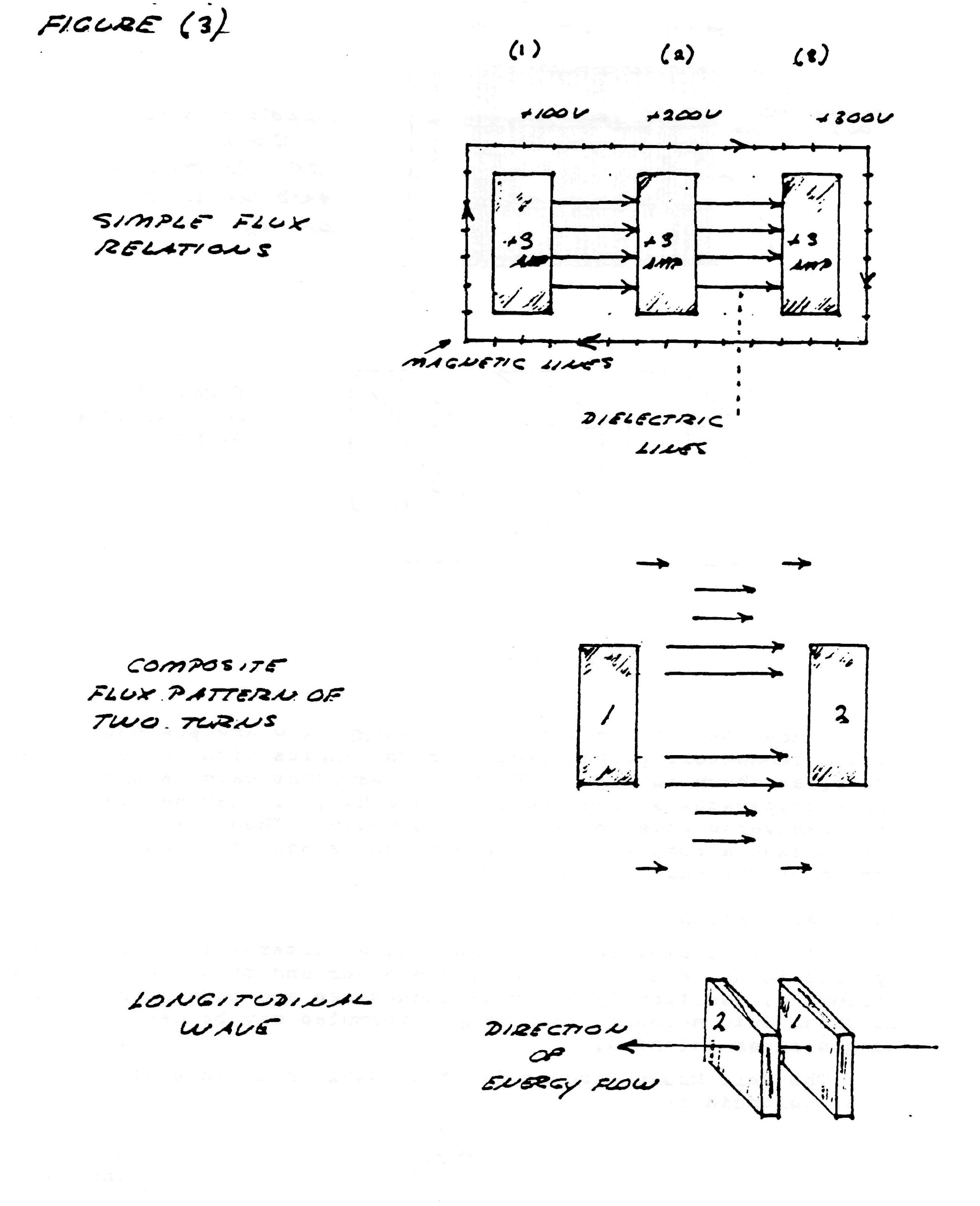
The apparatus of Fig. 3 produces a quite different wave form (Fig. 5). The mechanical force delivered to the shaft is applied at a right angle to the axis in clockwise direction. The counterforce is applied in the apposite rotational sense or counter-clockwise dir�ection at a right angle to the axis. The flow of mechanical energy is still along the shaft as in Fig. 4, however, it no longer pulsates in magnitude with the cycle but it continues, quite like the flow of electric energy in a direct current circuit,
An analogy is a screw and screwdriver. The screwdriver is forced rotationally clockwise by the hand or other motive force, The counter force appears in opposition, that is counterclockwise, thereby ar�resting the rotation of the screwdriver. However, the wood is soft and cannot reflect the counterforce back into the screwdriver. Thus the screw travels longitudinally into the wood, perpendicular to the rotation of the screwdriver. The form of this wave has been of great interest to a wide variety of fields of endeavor. It has been called the Caduceus coil, spinning wave, double helix, solar cross, and of course the rotating magnetic field. Applications are as wide ranging, from sewage treat�ment plants and guided missies all the way to the Van Tassel Integra�tron and astrology.
The Oscillating Current Transformer
Originally published in JBR, May-June 1986.
The Oscillating Current Transformer
The oscillating current transformer functions quite differently than a conventional transformer in that the law of dielectric in�duction is utilized as well as the familiar law of magnetic induct�ion. The propagation of waves along the coil axis does not resemble the propagation of waves along a conventional transmission line, but is complicated by inter-turn capacitance & mutual magnetic inductance. In this respect the O.C. transformer does not behave like a resonant transmission line, nor a R.C.L. circuit, but more like a special type of wave guide. Perhaps the most important feature of the O.C. transformer is that in the course of propa�gation along the coil axis the electric energy is dematerialized, that is, rendered mass free energy resembling Dr. Wilhelm Reich's Orgone Energy in its behavior. It is this feature that renders the O.C. transformer useful for wireless power transmission and reception, and gives the O.C. transformer singular importance in the study of Dr. Tesla's research.
FUNDAMENTALS OF COIL INDUCTION
Consider the elemental slice of a coil shown in fig. 1. Between the turns 1,2 & 3 of the coiled conductor exists a complex electric wave consisting of two basic components. In one component (fig. 2), the lines of magnetic and dielectric flux cross at right angles, producing a photon flux perpendicular to these crossings, hereby propagating energy along the gap, parallel to the conductors and around the coil. Th�s is the transverse electro-magnetic wave. In the other component, shown in fig. 3, the lines of magnetic flux do not cross but unite along the same axis, perpendicular to the coil conductors, hereby energy is conveyed along the coil axis. This is the Longitudinal Magneto-Dielectric Wave.
Figure (1)
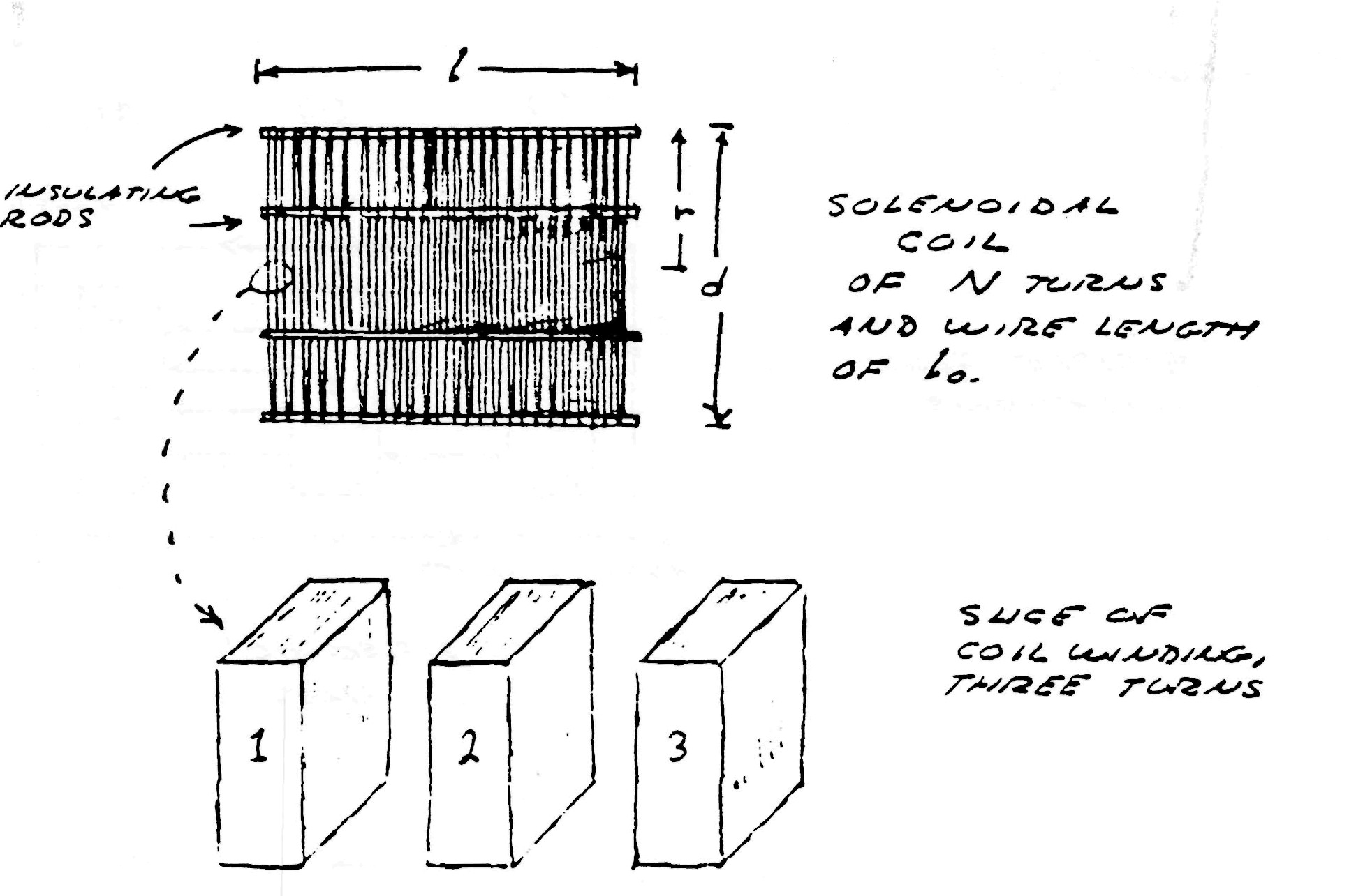
Figure (2)
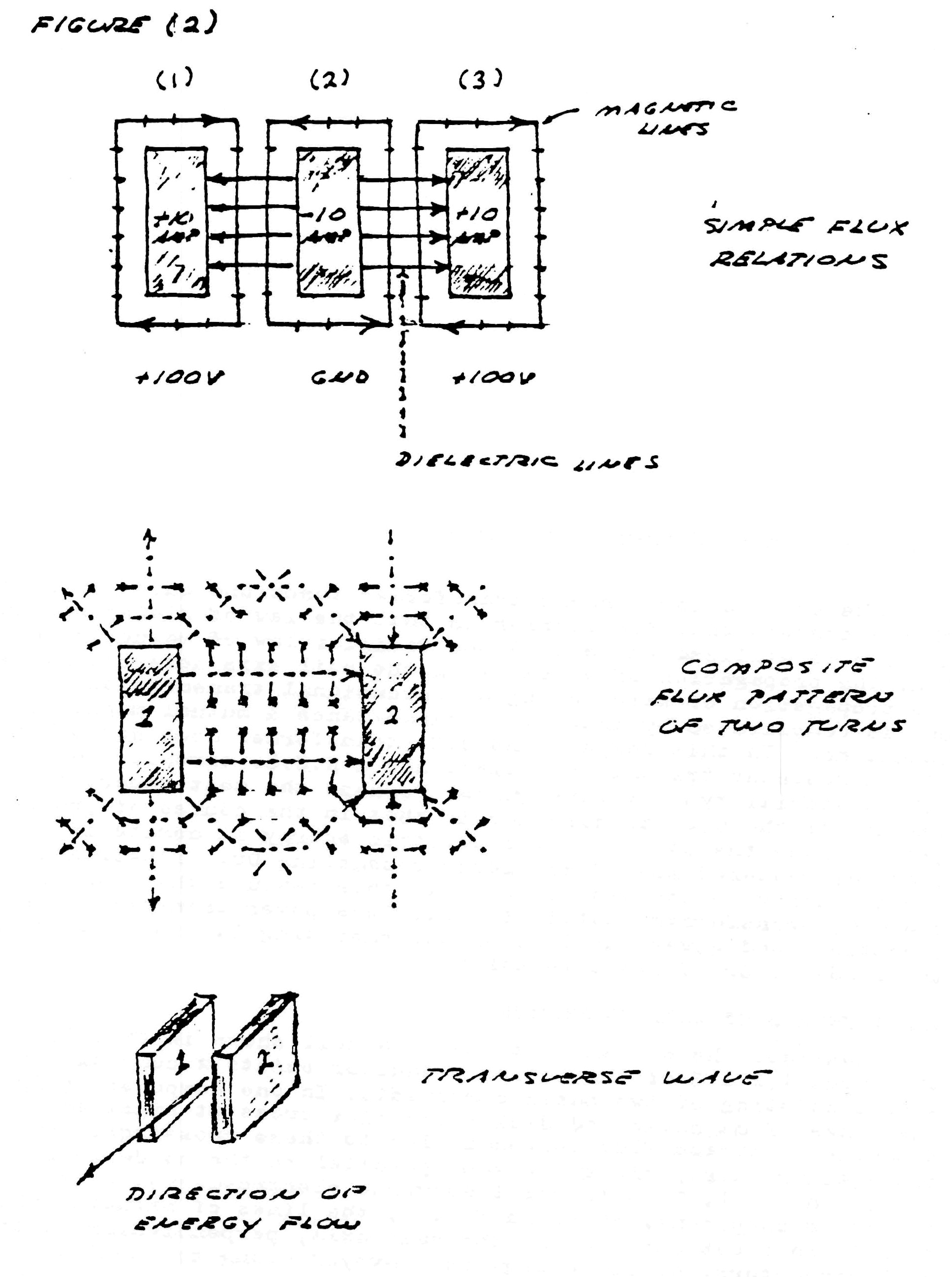
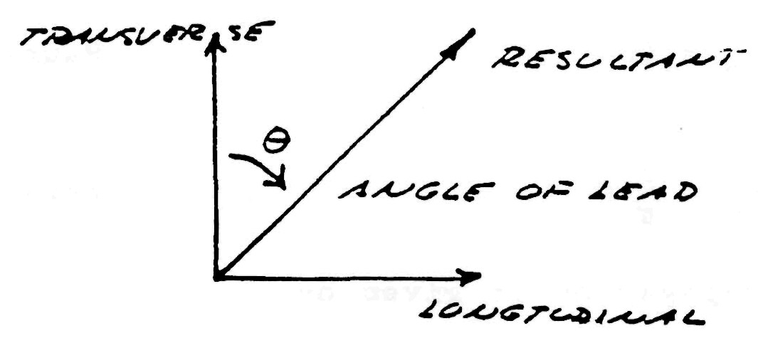
Hence, two distinct forms of energy flow are present in the coiled conductor, propagating at right angles with respect to each other, as shown in fig. 4. Hereby a resultant wave is produced which propagates around the coil in a helical fashion, leading the transverse wave between the conductors. Thus the oscillating coil posses a complex wavelength which is shorter than the wave�length of the coiled conductor.
COIL CALCULATION
If the assumptions are made that an alternating current is applied to one end of the coil, the other end of the coil is open circuited, Additionally external inductance and capacitance must be taken into account, then simple formulae may be derived for a single layer solenoid.
The well known formula for the total inductance of a single layer solenoid is
| $ L = \frac{r^2 N^2}{ (9r + 10l) }$ | $ x 10^{-6}$ Henry (inches) (1) |
Where:
- r is coil radius in inches
- l is coil length in inches
- N is number of turns
| $ L = \frac{31.6 r_1^2 N^2}{ (6 r_1 + 9l + 10(r_2-r_1)) }$ | microHenry |
| $ L = \frac{r^2 N^2}{ (8 r + 11w) }$ | microHenry |
Figure (3)
The capacitance of a single layer solenoid is given by the formula
| $C = pr$ | $ 2.54 x 10^{-12}$ Farads (inches) (2) |
where the factor p is a function of the length to diameter ratio, tabulated in table (1). The dimensions of the coil are shown in figure (1). The capacitance is minimum when length to diameter ratio is equal to one.
Because the coil is assumed to be in oscillation with a stand�ing wave, the current distribution along the coil is not uniform, but varies sinusoidially with respect to distance along the coil. This alters the results obtained by equation (1), thus for resonance
| $L_0 = \frac12 L$ | Henrys (3) |
likewise, for capacitance
| $C_0 = \frac{8}{\pi} C$ | Farads (4) |
Hereby the velocity of propagation is given by
| $\begin{eqnarray} V_0 & = & \frac{1}{\sqrt {L_0 C_0}} \\ & = & \eta V_c \end{eqnarray}$ | Units/sec (5) |
Where
| $ V_c = \frac{1}{\sqrt {\mu \epsilon}} $ | Inch/sec (6) |
That is, the velocity of light, and
| $\begin{eqnarray} V_0 & = & \eta V_c \\ & = & \left[ \begin{array}{cc} \frac{1.77}{p} + \frac{3.94}{p}n \end{array} \right]^\frac12 \end{eqnarray}$ | $2 \pi 10^9$ Inch/sec (7) |
Where n = the ratio of coil length to coil diameter. The values of propagation factor $\eta$ are tabulated in table (2).
| $ F_{res} = (0.39 * ln(h/d) + 1.19) * 75e6 / l $ | (Hertz) |
Thus, the frequency of oscillation or resonance of the coil is given by the relation
| $ F_0 = \frac{V_0}{ (l_0 . 4) } $ | Cycles/sec (8) |
Where $l_0$ = total length of the coiled conductor in inches.
Figure (4)
The characteristic impedance of the resonant coil is given by
| $ Z_c = \sqrt {\frac{L_0}{C_0}}$ | Ohms (9) |
Hence,
| $ Z_c = N Z_s $ | Ohms (10) |
Where
| $ Z_s = \left[ \begin{array}{cc} (182.9 + 406.4n)p \end{array} \right]^\frac12 $ | $ \frac{\pi}{2} 10^3$ Ohms (inches) (11) |
and N = number of turns. The values of sheet impedance, $Z_s$, are tabulated in table (3).
The time constant of the coil, that is, the rate of energy dissipation due to coil resistance is given by the approximate formula
| $ u = \frac{R_0}{2 L_0} = ( \frac{2.72}{r}+ \frac{2.13}{l}) \pi \sqrt{F_0} $ | Nepers/sec (inches) (12) |
Where
- r = coil radius
- l = coil length
In general, the dissipation of the coil's oscillating energy by conductor resistance:
- Decreases with increase of coil diameter, d;
- Decreases with increase of coil length, l, rapidly when the ratio, n, of length to diameter is small with little decrease beyond n equal to unity;
- Is minimum when the ratio of wire diameter to coil pitch is 60%.
By examination of the attached tables, (1), (2) & (3), it is seen that the long coils of popular designs do not result in optimum performance. In general, coils should be short and wide, and not longer than n=1. The frequency is usually given as $F_0 = V_c / \lambda_0$ which by equation (7) is incorrect. Winding on solid or continuous formers rather than spaced slender rods, as shown in figure (1), greatly retards wave propagation as indicated in equation (6), thereby seriously distorting the wave. The dielectric constant of the coil,$\epsilon$ , should be as close to unity as is physically possible to insure high efficiency of transformation.
The equations for the voltampere relations of the oscillating coil are
| $ \dot E_1 = j ( Z_c Y_0 + \delta) \dot E_0 $ | Complex Input Voltage (13) |
| $ \dot I_1 = j ( Y_c Z_0 + \delta) \dot I_0 $ | Complex Input Current (14) |
| $ Z_1 = \frac{Z_c Y_0 + \delta}{Y_c Z_0 +\delta} Z_0 $ | Input Impedance, Ohms (15) |
Where
- $ \dot E_0 = $ Voltage on elevated terminal
- $ \dot I_0 = $ Current into elevated terminal
- $ Y_c = Z_c^{-1}$
- $ Z_0 = $ Terminal impedance
- $ Y_0 = $ Terminal admittance
- $ \delta = \frac{u}{2 F_0} = $ Decrement
- $ j =$ root of $\sqrt{-1}$
For negligible losses and absolute values
| $ E_1 = ( Z_c 2 \pi F_0 C_0) E_0 $ | Volts (16) |
| $ I_1 = ( Y_c / 2 \pi F_0 C_0) I_0 $ | Amperes (17) |
Where
- $C_0 =$ Terminal capacitance
By the law of conservation of energy
| $ E_1 I_1 = E_0 I_0 $ | Volt-Amperes (18) |
If the terminal capacitance is small then the approximate input/ output relations of the Tesla coil are given by
| $ E_0 = Z_c I_1 $ | Output Volts (19) |
| $ I_1 = E_0 Y_c $ | Input Amperes (20) |
| $ I_0 = Y_c E_1 $ | Output Amperes (21) |
| $ E_1 = I_0 Z_c $ | Input Volts (22) |
TABLE (1) Coil Capacitance Factor
| Length/Width = n | Factor P | Length/Width = n | Factor P |
| 0.10 | 0.96 | 0.80 | 0.46 |
| 0.15 | 0.79 | 0.90 | 0.46 |
| 0.20 | 0.70 | 1.00 | 0.46 |
| 0.25 | 0.64 | 1.5 | 0.47 |
| 0.30 | 0.60 | 2.0 | 0.50 |
| 0.35 | 0.57 | 2.5 | 0.56 |
| 0.40 | 0.54 | 3.0 | 0.61 |
| 0.45 | 0.52 | 3.5 | 0.67 |
| 0.50 | 0.50 | 4.0 | 0.72 |
| 0.60 | 0.48 | 4.5 | 0.77 |
| 0.70 | 0.47 | 5.0 | 0.81 |
TABLE (2)
| Length/Width = n | $V_0$ Inches/Sec | Percent Luminal Velocity = $\eta$ |
| 0.10 | 9.42 x 10^9 | 79.8% |
| 0.15 | 10.9 | 92.2 |
| 0.20 | 12.0 | 102 |
| 0.25 | 13.0 | 110 |
| 0.30 | 13.9 | 118 |
| 0.35 | 14.8 | 125 |
| 0.40 | 15.6 | 132 |
| 0.45 | 16.4 | 139 |
| 0.50 | 17.2 | 146 |
| 0.60 | 18.4 | 156 |
| 0.70 | 19.5 | 165 |
| 0.80 | 20.5 | 176 |
| 0.90 | 21.4 | 181 |
| 1.00 | 22.1 | 187 |
| 1.5 | 25.4 | 215 |
| 2.0 | 27.6 | 234 |
| 2.5 | 28.7 | 243 |
| 3.0 | 29.7 | 251 |
| 3.5 | 30.3 | 257 |
| 4.0 | 30.9 | 262 |
| 4.5 | 31.6 | 268 |
| 5.0 | 32.4 | 274 |
| 6.0 | 33.0 | 279 |
| 7.0 | 33.9 | 287 |
TABLE (3)
| L/W =n | $Z_s$ |
| 0.10 | 0.107 x 10 |
| 0.15 | 0.070 |
| 0.20 | 0.116 |
| 0.25 | 0.116 |
| 0.30 | 0.116 |
| 0.35 | 0.115 |
| 0.40 | 0.115 |
| 0.45 | 0.114 |
| 0.50 | 0.113 |
| 0.60 | 0.110 |
| 0.70 | 0.106 |
| 0.80 | 0.103 |
| 0.90 | 0.099 |
| 1.00 | 0.095 |
| 1.5 | 0.081 |
| 2.0 | 0.070 |
| 2.5 | 0.061 |
| 3.0 | 0.054 |
| 3.5 | 0.048 |
| 4.0 | 0.044 |
| 4.5 | 0.040 |
| 5.0 | 0.037 |
| 6.0 | 0.032 |
| 7.0 | 0.028 |
Books by Eric Dollard
CONDENSED INTRO TO TESLA TRANSFORMERS. This book is an abstract of theory and construction techniques of Tesla transformers. It is the result of experimental investigations and theoretical considerations. Includes relevant Tesla patent and an article on capacity by Fritz Lowenstein, Tesla's assistant. (BSRA #TE-1)
INTRODUCTION TO DIELECTRIC & MAGNETIC DISCHARGES IN ELECTRICAL WINDINGS, Theory of abrupt electrical oscillations such as those used by Tesla for experimental researches. Contains ELECTRICAL OSCILLA� TIONS IN ANTENNAE AND INDUCTION COILS by John Miller, 1919. This is one of the few articles containing equations useful to the design of Tesla coils. (BSRA #TE-2)